In this tutorial we explore the working principle of the thermometer using a rich set of laboratory tools.
Contents
Materials
- Water
- Food coloring
Equipment
- Metal base PS2030.27
- Metal support rod PS2030.28
- Metal rod with metal clamp PS2030.30
- 2 bosses PS2030.29
- Retort ring & gauze PS2030.31, PS2030.32
- Glass beaker 400 ml PS2030.5
- Round bottomed flask PS2030.19
- Delivery tube PS2030.20
- Beaker clamp PS2030.15
- Alcohol burner PS2030.25
- Lighter CS3001.35
- Ruler PS2021.18
- Temperature sensor RS104
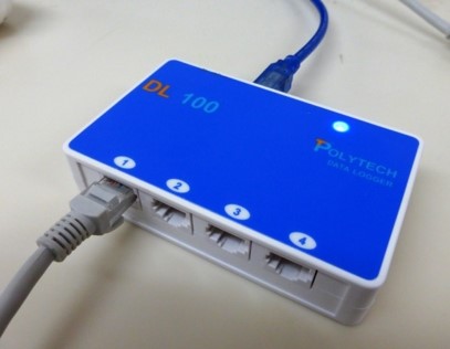
- Data logger DL100
- Windows PC with iLab software

Safety Note
No personal safety requirements for this experiment.
For the proper usage of the Temperature sensor please read the instruction manual before.
- Connect the DL100 data logger with the PC and the temperature sensor
- a. Dowload the experiment files
b. Run the iLab software
c. Open the experiment file: T-D.dis using iLab
– OR –
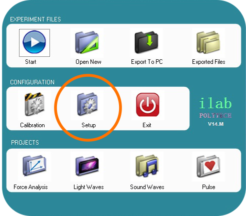
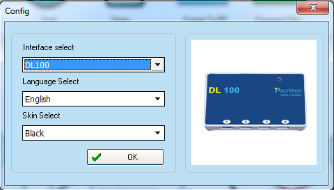
- d. Run the iLab software and in the main menu select «Setup» (pic. 1). Make sure that the “DL100” option is already chosen.(pic. 2)
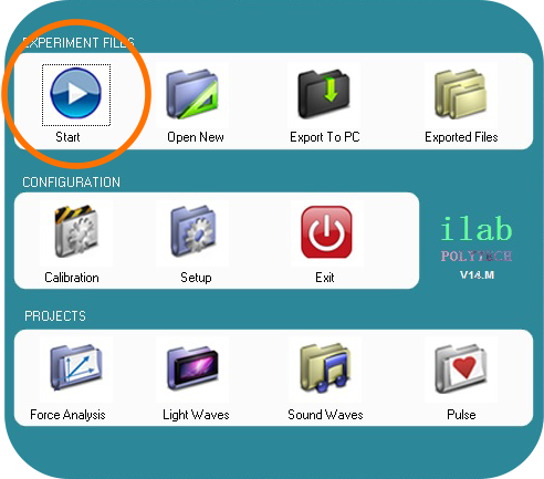
- In the main menu select “Start” and the experiment screen will open automatically.
- In the experiment screen you can see the following functional areas:
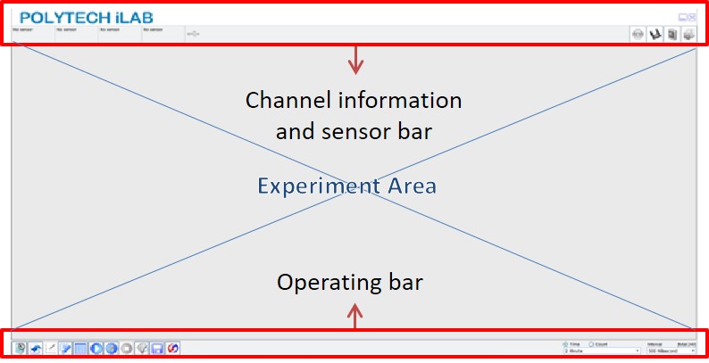
- On the operation bar select «Rapid experiment (F1)“. The experiment screen will open with options for configuring the variables temperature (T) and time (s) on the axes.

- Whenever you are ready select “Manually (F7)” to start recording the first measurement and by clicking on the same button you can take the second measurement.

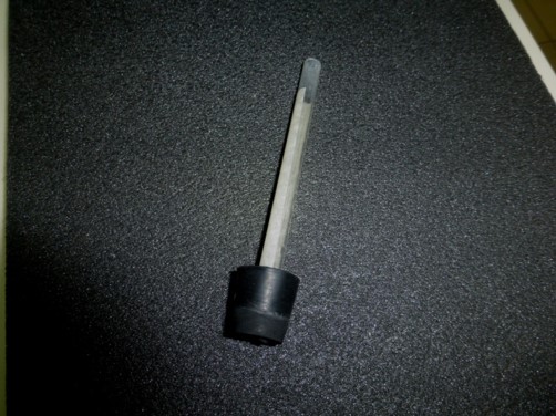
- Stick a piece of paper (or paper tape) on the delivery tube and attach the delivery tube into the hole of the big sized rubber bang. (see the picture)
- You can prepare the water by heating it into the glass beaker 400 ml and adding a few drops of food coloring.
- Set up the metal base, the retort ring with gauze and the metal clamp according to the picture.
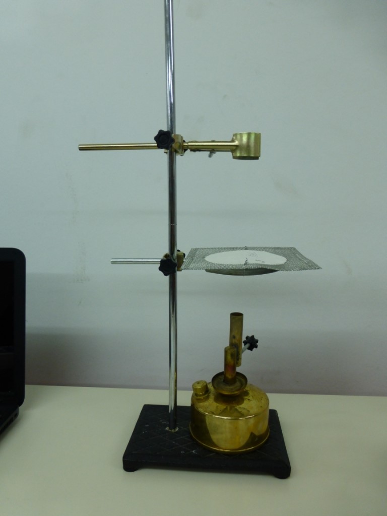
- Place the alcohol burner on the metal base.
- Add (heated) water into the round bottomed flask and adjust the flask to the metal clamp. Seal the flask with the rubber cap.
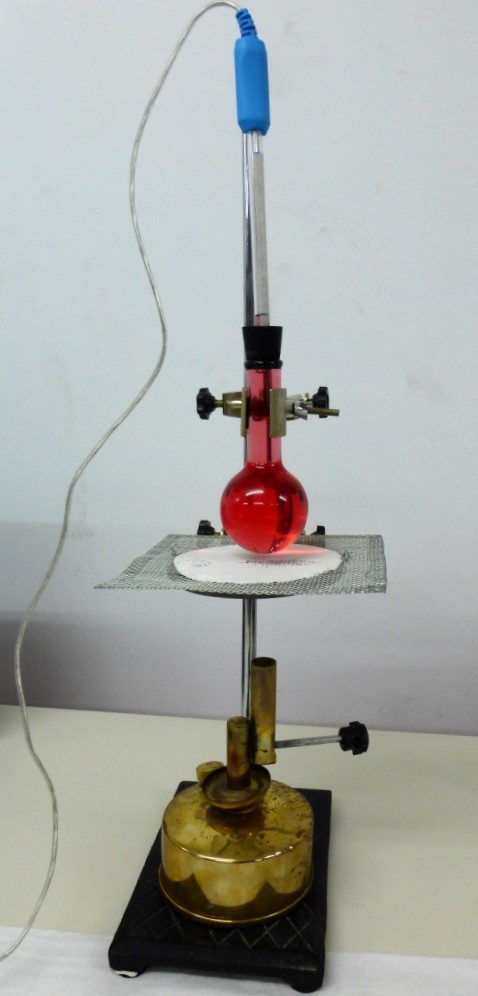
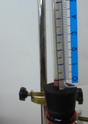
- Insert the temperature sensor probe into the delivery tube. The water level will rise and it will appear to the tube. (Add a few drops of water if necessary).
- With a ruler and a pen mark the water level in the tube, drawing a line on the paper you stuck in step 7.
- Then, per half a centimeter draw a line.
- Turn on the alcohol burner and on the iLab select “Manually (F7)” to take the first measurement before the volume changes.
- Whenever the water level increases by half a centimeter (reaches the next line you marked on the paper) press again “Manually (F7)” to take the next measurement.
At the end you will have a graph like the one in the image. However the graph is not useful for your calculation because you need a level of water-temperature graph and not a time-temperature graph.
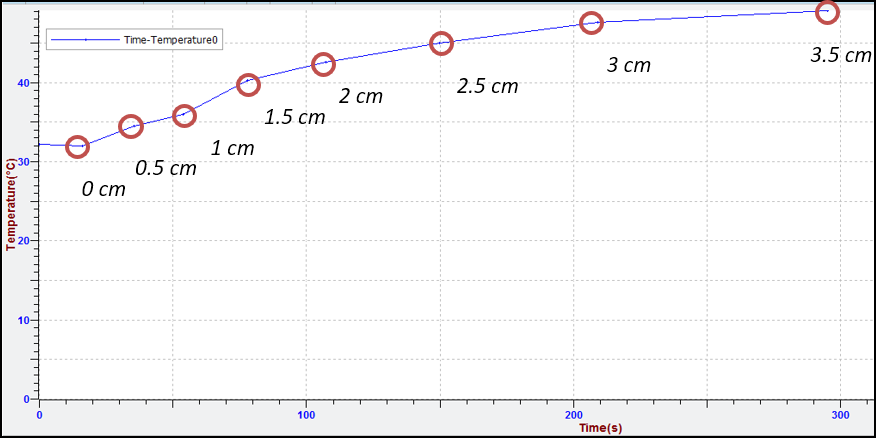
Note: You can find our measurements in the experiment file T-T.dis that you downloaded in step 2.a.
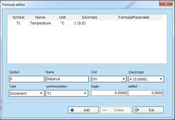
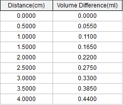
- You know that every measure you made was when the fluid level increased by 0.5 cm. You will therefore introduce a new parameter that reflects the height of the tube in centimeters.
Select “Edit variable (F4)” and fill the fields in the formula editor window like the picture.

- To create the Distance(cm) – Temperature (°C) graph:
- select “Add line (F3)”

- delete the temperature-time graph
- add the new graph by selecting Distance at x-axis and Temperature at y-axis.
- select “Add line (F3)”
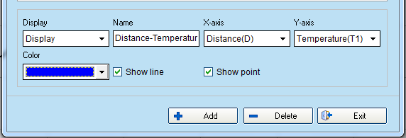
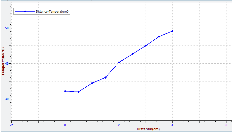
- The graph should be similar to the image. Select “Data table (F5)”
 to see details for the points of the curve. Do you believe that through these points must calibrate your thermometer?
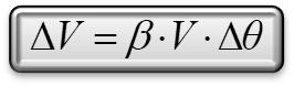
The dependence of the volume change of the liquid in relation to temperature is linear, as we know from the mathematical expression that describes it:
ΔV volume change, V initial volume, ΔΘ temperature change and β the expansion coefficient.Therefore, for every temperature change there is an equivalent volume change. Because of metric errors this is not completely described by the chart.
- Select “curve management”
 and then make linear regression to the curve.
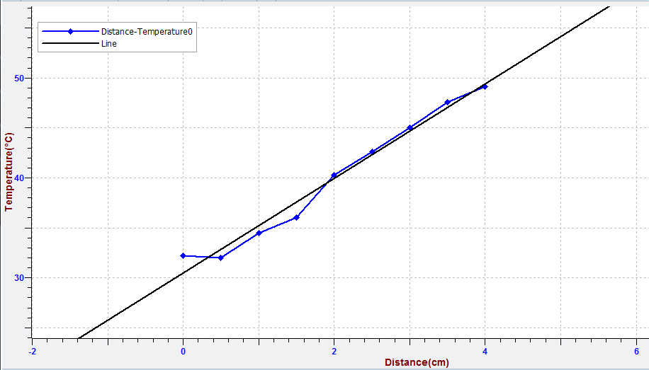
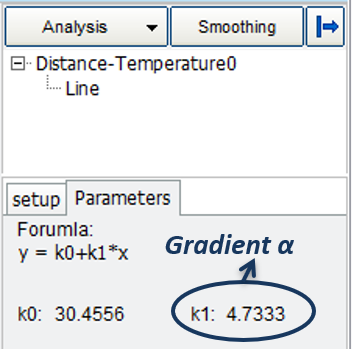
With a very good approximation we can assume that prices on a straight line can be expressed by the formula: y = αx + β.
The gradient of the line α describes the rate of change of temperature with respect to the liquid level in the tube.
- Fill in the gradient α into the “curve management” and draw a proper calibration of the thermometer that you created.
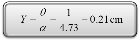
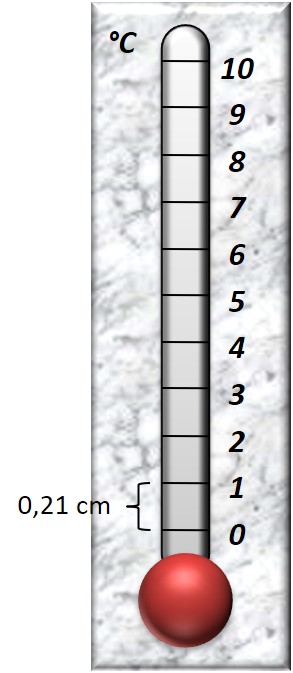
Suppose that in the calibration you want:
θ = 0 °C at the point 0 of our curve. Then temperature θ = 1°C will be drawn at distance Υ from 0, where Υ:
Question 1
The temperature of a body is a physical quantity that shows us how hot or cold is the body.
- True
- False
Question 2
Measuring temperature is important for
- health.
- food preservation.
- function of devices and machines.
- All the above.
Question 3
The thermometer is calibrated by recording the indication of the time a piece of ice is converted into water and the indication of when the water starts to boil and is converted to vapor.
- The first indication corresponds to 0°C (melting) and the second to 100°C (boiling point).
- The first indication corresponds to 4°C (melting) and the second to 100°C (boiling point).
- The first indication corresponds to 0°C (boiling point) and the second to 100°C (melting).
- The indications depend every time on the quantity of water and ice.
Question 4
What is the right way of looking the record of a thermometer?
- Vertical to the thermometer and at a short distance from it.
- Vertical to the thermometer and at distance from it.
- Touching the thermometer by hand in order to have more accurate observation.
- Angled to be more distinct indication.
Question 5
Water is liquid. After boiling and evaporation remains in the same physical state?
- Yes
- No
End of tutorial